Generate Dynamic Images from Google Sheets — No Code Required

Ever wished you could generate hundreds of personalized images directly from a spreadsheet? Now you can! With SnapShark's new Google Sheets integration, you can turn any row of data into a beautifully designed image — automatically.

Whether you're creating social media graphics, product images, personalized certificates, or event invitations, this integration lets you go from spreadsheet to finished images in minutes. No coding required.

✨ What You Can Do

• Generate bulk images from spreadsheet rows — no coding needed
• Automatically pull template variables into column headers
• Render images one-by-one or all at once with a single click
• Get direct CDN links to your generated images
• Change text, swap photos, and personalize every single image
• Works with any SnapShark template you've created

---

🛠️ Setup Guide

Setting up the integration takes about 5 minutes. Here's everything you need to do:

Step 1: Select Your Template & Generate an API Token

Head over to Settings → Integrations in your SnapShark dashboard. You'll see the Google Sheets card — click to expand it.

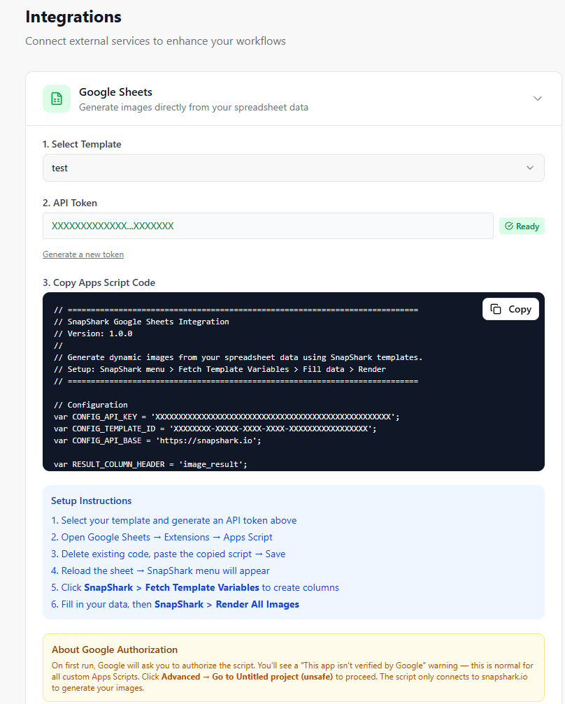
Choose your template from the dropdown — this is the design you'll use to generate images. Then click "Generate Token for Google Sheets" to create a secure API token. This token lets the script communicate with SnapShark on your behalf.

Your API token and template selection are saved automatically. You won't need to regenerate them every time you visit this page.

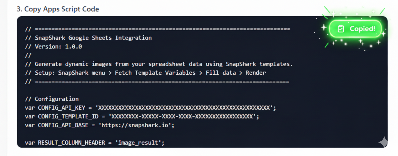
Step 2: Copy the Apps Script Code

Once you've selected a template and generated a token, the pre-configured script code appears below. Your API token and template ID are already embedded — no manual editing needed!

Click the "Copy" button in the top-right corner of the code block.

Step 3: Paste into Google Sheets

1. Open Google Sheets and create a new spreadsheet (or open an existing one)
2. Go to Extensions → Apps Script

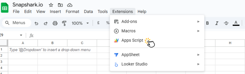
3. Delete any existing code in the editor
4. Paste the copied script code
5. Click Save (or press Ctrl+S)

Step 3.5: Save & Authorize the Script (One-Time Setup)

Before using the script, you need to save it to your Google Drive and grant the required permissions. This is a one-time process.

1. After pasting the code, click the "Save project to Drive" button (💾 icon) next to the Run button at the top of the Apps Script editor. You can also press Ctrl+S.
2. Now click Run to trigger the authorization flow.
3. A popup will appear saying "Authorization required". Click "Review permissions".
4. Select your Google account to continue.
5. You'll see a warning: "Google hasn't verified this app" — this is completely normal for all custom Apps Scripts. Click "Advanced" at the bottom left.
6. Click "Go to Untitled project (unsafe)" to proceed. Don't worry — the script only connects to snapshark.io to generate your images.
7. On the permissions screen, click "Select all" to grant all required permissions, then click "Continue".

That's it! The authorization is done — you won't need to repeat this process again.

8. Close the Apps Script tab and reload your spreadsheet
9. After a few seconds, you'll see the SnapShark menu appear in the menu bar!

Step 4: Fetch Template Variables

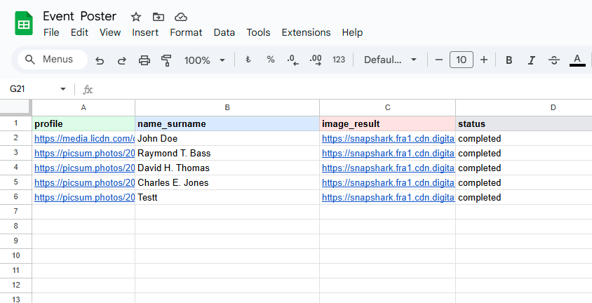
Click SnapShark → Fetch Template Variables from the menu. The script will connect to SnapShark, fetch your template's dynamic variables, and automatically create color-coded column headers in your sheet.

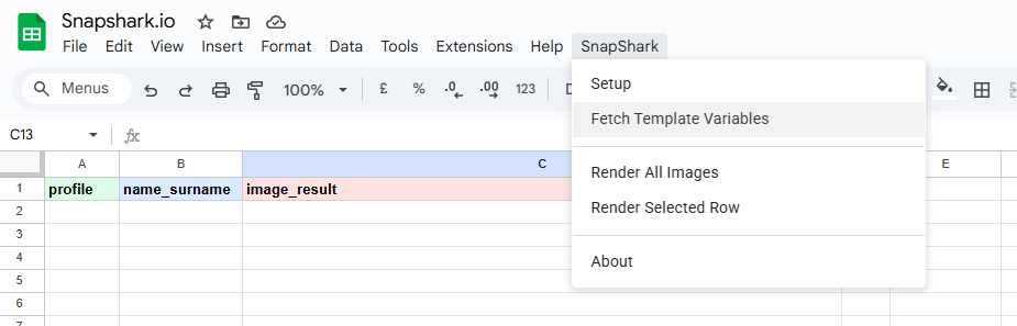
Here's what the colors mean:

Color	Meaning
🔵 Blue	Text variables — headlines, descriptions, names, etc.
🟢 Green	Image variables — photos, logos, background images
🔴 Red	image_result — the generated image URL appears here
⚪ Gray	status — shows rendering progress and errors

Step 5: Fill In Your Data

Now the fun part! Fill in your rows with the content you want in each image:

• Text columns: Type your text — headlines, names, descriptions, prices, anything
• Image columns: Paste publicly accessible image URLs

Each row becomes one image. Add as many rows as you need!

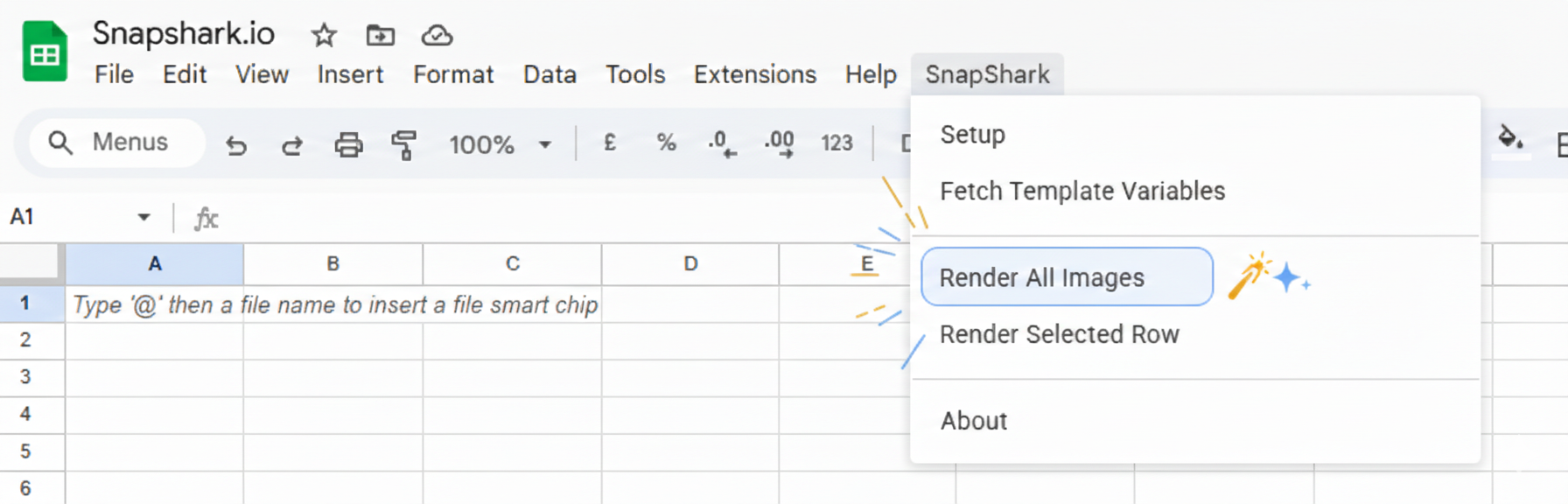
Step 6: Render Your Images 🚀

You have two options:

Option A: Render All Images — Click SnapShark → Render All Images to process every row that doesn't have a result yet. The script will ask for confirmation, then render each row one by one, showing progress toasts along the way.

Option B: Render Selected Row — Click on any single data row, then choose SnapShark → Render Selected Row. Perfect for testing a single row before doing a full batch.

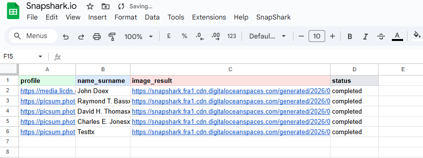
That's it! Your generated image URLs are now in the image_result column, ready to use anywhere.

---

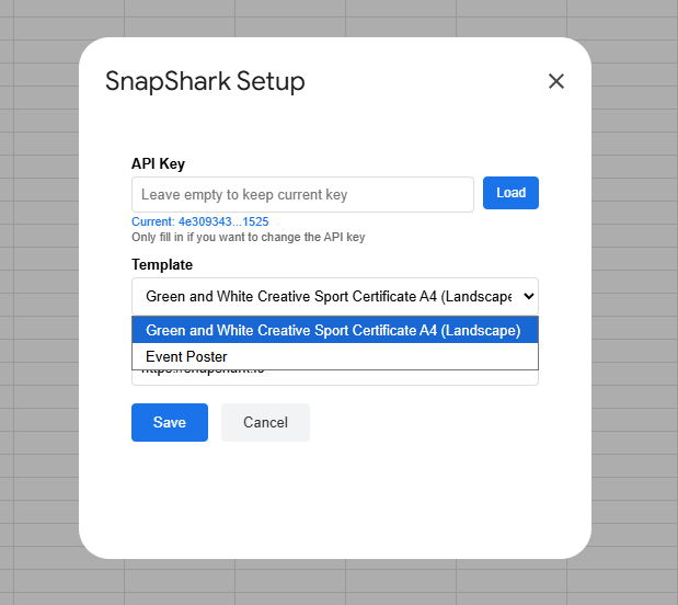
🔄 Changing Templates or API Token

Need to switch to a different template or update your API key? You don't need to re-copy the entire script.

Just click SnapShark → Setup in the menu to open the configuration dialog right inside Google Sheets. The dialog connects to your SnapShark account and shows all your templates in a dropdown list — no need to manually copy Template IDs.

When you select a different template and save, the script automatically creates a new sheet tab named after that template and sets up the column headers for you. Each template gets its own tab, keeping your data organized.

---

💡 Tips & Best Practices

Template Design Tips

• Give your template layers clear, descriptive names (e.g., "headline", "photo", "subtitle") — these become your column headers automatically
• Use text and image variable types for the best Google Sheets experience
• Set default values in your template — they'll appear as sample data in the sheet

Spreadsheet Tips

• Keep your data clean — empty cells are skipped during rendering
• The image_result column is your output — don't edit it manually
• Want to re-render a row? Just clear its image_result cell and run Render again
• You can use Google Sheets formulas to generate dynamic values! (e.g., =CONCAT(A2, " - ", B2))

Performance Notes

• Google Apps Script has a 6-minute execution limit — this comfortably handles ~100–150 images per batch
• For larger batches, just run Render All Images multiple times — it automatically skips rows that already have results
• There's a 500ms delay between renders to ensure stability

---

🧩 How It Works Behind the Scenes

Here's the flow every time you render an image:

1. The script reads your column headers and the current row's data
2. It builds an API request that maps each column to its template variable
3. The request is sent to SnapShark's image generation API with your API token
4. SnapShark renders the image server-side using your template + the row data
5. The CDN URL of the finished image is written back to the image_result column

Your API token authenticates every request, ensuring only you can access your templates and use your credits.

---

❓ Frequently Asked Questions

How many images can I generate at once?
As many as your credits allow. The script processes rows sequentially with a small delay to ensure reliability. For very large batches (500+), just run the render command multiple times.

Do I need to know how to code?
Not at all. Everything is copy-paste — the script comes pre-configured with your API token and template ID.

Can I use any image URL in image columns?
Yes, as long as the image is publicly accessible (no login required to view it). Direct URLs from image hosting services, CDNs, or public cloud storage all work great.

What happens if I run out of credits mid-render?
The script will mark that row with an "Insufficient credits" error in the status column and continue to the next row. You can add more credits and re-render the failed rows later.

Can multiple people use the same spreadsheet?
Yes! Each user can set their own API token via the SnapShark → Setup menu. The token is stored per-user, so multiple team members can share the same sheet.

---

🚀 Get Started Now

Ready to generate images from your spreadsheet? Here's your quick checklist:

1. Go to Settings → Integrations in your SnapShark dashboard
2. Expand the Google Sheets card
3. Select your template, generate a token, and copy the script
4. Paste it into Google Sheets and start rendering!

If you haven't created a template yet, head over to the template editor to design one first. Once your template is ready, the Google Sheets integration is just a few clicks away.

Happy generating! 🎉